Memorylessness

The hook

A radioactive atom has been sitting in a laboratory for a million years without decaying. Is it “due” to decay soon? No: its chance of decaying in the next second is exactly the same as that of a freshly made atom. Radioactive atoms do not age. The waiting time until decay has the exponential distribution, and its defining property is that it has no memory.

This question shows the memorylessness in a striking form. Split an exponential waiting time into its whole number of units and its fractional part. These two pieces turn out to be independent: knowing how many whole hours you waited tells you nothing about the minutes. The question also explains, in the exercises, why your wait for a bus can seem longer than the gap between buses.

Before you start

\(\mathrm{P}(X > x) = \int_x^\infty\lambda e^{-\lambda u}\,\mathrm{d}u = e^{-\lambda x}\). Then \(\mathrm{P}(X > s + t \mid X > s) = \frac{e^{-\lambda(s + t)}}{e^{-\lambda s}} = e^{-\lambda t} = \mathrm{P}(X > t)\): having already waited \(s\), the remaining wait has the same distribution as a fresh one. This is the memoryless property.

Working it through

Stage 1 The whole part

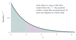
\(Y = n\) exactly when \(n \leq X < n + 1\): \[\mathrm{P}(Y = n) = e^{-\lambda n} - e^{-\lambda(n + 1)} = (1 - e^{-\lambda})e^{-n\lambda}. \qed\] So \(Y\) has a geometric distribution: each whole unit is “survived” with probability \(e^{-\lambda}\).

Stage 2 The fractional part

\[\mathrm{P}(Z < z) = \sum_{n \geq 0}\bigl(e^{-\lambda n} - e^{-\lambda(n + z)}\bigr) = (1 - e^{-\lambda z})\sum_{n \geq 0}e^{-\lambda n} = \frac{1 - e^{-\lambda z}}{1 - e^{-\lambda}}. \qed\]

Stage 3 The mean of \(Z\)

With \(c = 1 - e^{-\lambda}\), \(\mathrm{P}(Z > z) = 1 - \frac{1 - e^{-\lambda z}}{c}\), so \[\mathrm{E}(Z) = 1 - \frac1c\Bigl(1 - \frac{1 - e^{-\lambda}}{\lambda}\Bigr) = 1 - \frac1c + \frac1\lambda = \frac1\lambda - \frac{e^{-\lambda}}{1 - e^{-\lambda}} = \frac1\lambda - \frac{1}{e^\lambda - 1}. \qed\] (For small \(\lambda\), long waits, this tends to \(\frac12\): the fractional part is nearly uniform. For large \(\lambda\) it is close to \(\frac1\lambda\), because \(X\) is almost always less than \(1\).)

Stage 4 Independence

\[\mathrm{P}(Y = n, z_1 < Z < z_2) = \mathrm{P}(n + z_1 < X < n + z_2) = e^{-\lambda n}\bigl(e^{-\lambda z_1} - e^{-\lambda z_2}\bigr).\]

From (i) and (ii), \(\mathrm{P}(Y = n)\mathrm{P}(z_1 < Z < z_2) = (1 - e^{-\lambda})e^{-n\lambda}\cdot\frac{e^{-\lambda z_1} - e^{-\lambda z_2}}{1 - e^{-\lambda}}\), which is the same. So \(Y\) and \(Z\) are independent.■

Looking back

• Sum over pieces. Both the distribution of \(Z\) and the joint probabilities came from adding probabilities over the intervals \([n, n + 1)\).

• The tail formula. \(\mathrm{E}(Z) = \int\mathrm{P}(Z > z)\,\mathrm{d}z\) avoided finding the density.

• Factorisation means independence. The joint probability split into a function of \(n\) times a function of \(z_1\), \(z_2\).

What’s really going on

Why the exponential is special

The independence of \(Y\) and \(Z\) comes straight from \(e^{-\lambda(n + z)} = e^{-\lambda n}e^{-\lambda z}\), and that is the memoryless property in disguise. In fact the exponential is the only continuous distribution without memory: if \(\mathrm{P}(X > s + t) = \mathrm{P}(X > s)\mathrm{P}(X > t)\) for all \(s, t \geq 0\), then \(g(t) = \ln\mathrm{P}(X > t)\) satisfies \(g(s + t) = g(s) + g(t)\), and (for a monotonic \(g\)) this forces \(g(t) = -\lambda t\). That is why the exponential models waiting times for events that happen “at random”, with no build-up: radioactive decays, the arrival of customers, the failure of electronic components that do not wear out.

Minima and the waiting-time paradox

If \(X_1\) and \(X_2\) are independent exponentials with rates \(\lambda_1\) and \(\lambda_2\), then \(\mathrm{P}(\min > x) = e^{-\lambda_1x}e^{-\lambda_2x}\), so the minimum is exponential with rate \(\lambda_1 + \lambda_2\). Waiting for the first of two independent random events is like waiting for one event at the combined rate (STEP III 2002 Q13, in the exercises). Memorylessness also explains the waiting-time paradox: if buses arrive at random with an average gap of \(10\) minutes, then a passenger arriving at a random time waits on average \(10\) minutes, not \(5\), because the remaining wait is memoryless; and the gap they arrive in is on average \(20\) minutes long, since long gaps are more likely to be landed in.

The thinking skill

Try this next

Further reading

• Geoffrey Grimmett & Dominic Welsh, Probability: An Introduction (Oxford University Press), on the exponential distribution and the Poisson process.

• Sheldon Ross, Introduction to Probability Models (Academic Press). Exponential distributions, Poisson processes and queues.

• David Spiegelhalter, The Art of Uncertainty (Pelican). Randomness and waiting in everyday life.