The diagnostic test AL has a probability \(0.9\) of giving a positive result when applied to a person suffering from the rare disease mathematitis. It also has a probability \(1/11\) of giving a false positive result when applied to a non-sufferer. It is known that only \(1\%\) of the population suffer from the disease. Given that the test AL is positive when applied to Frankie, who is chosen at random from the population, what is the probability that Frankie is a sufferer?
In an attempt to identify sufferers more accurately, a second diagnostic test STEP is given to those for whom the test AL gave a positive result. The probability of STEP giving a positive result on a sufferer is \(0.9\), and the probability that it gives a false positive result on a non-sufferer is \(p\). Half of those for whom AL was positive and on whom STEP then also gives a positive result are sufferers. Find \(p\).
The hook
A test for a disease is \(90\%\) accurate on people who have it and gives few false alarms. Frankie tests positive. How worried should Frankie be? Most people, including, in many studies, most doctors, say “about \(90\%\)”. The true answer in this question is \(\frac{1}{11}\), about \(9\%\). Ten times smaller.
The mistake is to ignore the base rate: the disease is rare, so even a small false-positive rate among the many healthy people produces far more false alarms than there are true cases. This base-rate fallacy matters in medicine, in law (where it is called the prosecutor’s fallacy), in security screening and in machine learning. Bayes’ theorem is the cure.
Before you start
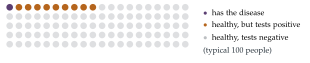
Imagine \(1000\) people. How many have the disease? How many of them test positive? How many of the healthy people test positive?
Of \(1000\) people, \(10\) have the disease and \(9\) of them test positive. Of the \(990\) healthy people, \(\frac{1}{11}\) test positive: \(90\) false positives. So \(99\) people test positive, of whom only \(9\) are ill.
Working it through
Stage 1 Bayes’ theorem
Write \(D\) for “Frankie has the disease” and \(+\) for “AL is positive”. You know \(\mathrm{P}(+ \mid D)\) and want \(\mathrm{P}(D \mid +)\). How are they related?
By the definition of conditional probability, \(\mathrm{P}(D \mid +) = \frac{\mathrm{P}(D \cap +)}{\mathrm{P}(+)}\), and \(\mathrm{P}(+)\) splits according to whether Frankie has the disease: \[\begin{aligned} \mathrm{P}(D \mid +) &= \frac{\mathrm{P}(+ \mid D)\mathrm{P}(D)}{\mathrm{P}(+ \mid D)\mathrm{P}(D) + \mathrm{P}(+ \mid \bar D)\mathrm{P}(\bar D)} \\ &= \frac{0.9 \times 0.01}{0.9 \times 0.01 + \frac{1}{11} \times 0.99} = \frac{0.009}{0.009 + 0.09} = \frac{1}{11}. \qed \end{aligned}\] This is the \(\frac{9}{99}\) of the thousand people.
Stage 2 A second test
The second test is given only to those who tested positive on AL. What is the proportion of sufferers in that group? Use it as the new “base rate”.
Among those positive on AL, a fraction \(\frac{1}{11}\) are sufferers and \(\frac{10}{11}\) are not. Applying Bayes’ theorem again, with these as the prior probabilities, \[\mathrm{P}(D \mid \text{both positive}) = \frac{0.9 \times \frac{1}{11}}{0.9 \times \frac{1}{11} + p \times \frac{10}{11}} = \frac{0.9}{0.9 + 10p}.\] Setting this equal to \(\frac12\) gives \(10p = 0.9\), so \(p = 0.09\).■
(Assuming, as the question implicitly does, that the two tests’ errors are independent given whether Frankie is ill.)
With \(p = 0.09\), STEP’s false-positive rate is about the same as AL’s, yet a second positive result raises the probability from \(\frac{1}{11}\) to \(\frac12\). Why does the same quality of test have a much bigger effect the second time?
Looking back
Natural frequencies. Imagining \(1000\) people made the answer obvious and easy to check.
Prior times likelihood. The posterior probability depends on both the test’s accuracy and the base rate.
Updating in stages. Yesterday’s posterior is today’s prior: the second test started from \(\frac{1}{11}\), not \(\frac{1}{100}\).
What’s really going on
Odds and evidence
Bayes’ theorem is clearest in terms of odds. The odds of \(D\) are \(\mathrm{P}(D) : \mathrm{P}(\bar D)\). A piece of evidence \(E\) multiplies the odds by the likelihood ratio \(\frac{\mathrm{P}(E \mid D)}{\mathrm{P}(E \mid \bar D)}\): \[\text{posterior odds} = \text{prior odds} \times \text{likelihood ratio}.\] Here the prior odds are \(1 : 99\), and AL’s likelihood ratio is \(0.9 \div \frac{1}{11} = 9.9\), giving posterior odds \(9.9 : 99 = 1 : 10\), that is, probability \(\frac{1}{11}\). A second independent test with likelihood ratio \(10\) (as STEP with \(p = 0.09\) has) brings the odds to \(1 : 1\). Taking logarithms, evidence adds: each independent test contributes the logarithm of its likelihood ratio. Alan Turing used exactly this, measuring evidence in “bans” and “decibans”, to break Enigma messages at Bletchley Park.
The prosecutor’s fallacy
In 1999 the solicitor Sally Clark was convicted of murdering her two baby sons, partly on the strength of evidence that the chance of two cot deaths in one family was “1 in 73 million”. Quite apart from the error in that number (it assumed the two deaths were independent, ignoring genetic and environmental factors), the reasoning confused \(\mathrm{P}(\text{evidence} \mid \text{innocent})\) with \(\mathrm{P}(\text{innocent} \mid \text{evidence})\). Double murder by a mother is also extremely rare, and the relevant comparison is between the two explanations. The Royal Statistical Society wrote publicly to point out the error, and her conviction was overturned in 2003. The mathematics is exactly that of this question.
In the 1990s the psychologist Gerd Gigerenzer showed that doctors who were given test statistics as conditional probabilities mostly got questions like this one badly wrong, but that when the same information was presented as natural frequencies (“of \(1000\) women, \(10\) have breast cancer; of these, \(8\) test positive…”) most got them right. His work has changed how medical risks are communicated to patients in many countries.
The thinking skill
\(\mathrm{P}(A \mid B)\) and \(\mathrm{P}(B \mid A)\) are different numbers. To get from one to the other you need the base rate \(\mathrm{P}(A)\).
Bayesian reasoning, updating beliefs in the light of evidence, is the foundation of modern statistics and machine learning, from spam filters to medical diagnosis. At university you will meet it as Bayesian inference, with prior and posterior distributions instead of single probabilities.
Try this next
A body in the fridge. (From STEP II, 1987.) Two friends, who tell the truth independently with probabilities \(p\) and \(q\), both tell me there is a body in my fridge. If I had thought this equally likely as not, explain why my new estimate should be \(\frac{pq}{1 - p - q + 2pq}\). There is indeed a body. It could be my enemy \(A\), my enemy \(B\), or both, which I judged equally likely; both friends now say \(A\) is in the fridge. What is my new estimate that both are there?
How rare? For a test with sensitivity \(0.9\) and false-positive rate \(\frac{1}{11}\), how common must a disease be for a positive result to mean a better than even chance of having it?
Repeat the test. If AL itself is repeated, and the results are independent given the person’s true state, what is the probability of disease after two positive AL results? After three?
Screening. A screening programme tests a million people for a condition with prevalence \(1\) in \(10\,000\), using a test with sensitivity \(99\%\) and false-positive rate \(1\%\). How many people will be told they may have the condition, and how many of them actually do?
Further reading
Gerd Gigerenzer, Reckoning with Risk (Penguin). Natural frequencies, medical tests and the courtroom.
David Spiegelhalter, The Art of Statistics (Pelican). Includes medical screening and the Sally Clark case.
Sharon Bertsch McGrayne, The Theory That Would Not Die (Yale University Press). The history of Bayes’ theorem, including Turing’s use of it.